Introduction and geometric constructions

Engineering drawing


Technical drawings

An engineering drawing, a type of technical drawing, is used to fully and clearly define requirements for engineered items.

Engineering drawing (the activity) produces engineering drawings (the documents). More than merely the drawing of pictures, it is also a language—a graphical language that communicates ideas and information from one mind to another.[1] Most especially, it communicates all needed information from the engineer who designed a part to the workers who will make it.


Overview 

Relationship to artistic drawing 

Engineering drawing and artistic drawing are both types of drawing, and either may be called simply "drawing" when the context is implicit. Engineering drawing shares some traits with artistic drawing in that both create pictures. But whereas the purpose of artistic drawing is to convey emotion or artistic sensitivity in some way (subjective impressions), the purpose of engineering drawing is to convey information (objective facts).  One of the corollaries that follows from this fact is that, whereas anyone can appreciate artistic drawing (even if each viewer has his own unique appreciation), engineering drawing requires some training to understand (like any language); but there is also a high degree of objective commonality in the interpretation (also like other languages).  In fact, engineering drawing has evolved into a language that is more precise and unambiguous thannatural languages; in this sense it is closer to a programming language in its communication ability. Engineering drawing uses an extensive set of conventions to convey information very precisely, with very little ambiguity.

Relationship to other technical drawing types 

The process of producing engineering drawings, and the skill of producing those, is often referred to as technical drawing or drafting (also spelled draughting), although technical drawings are also required for disciplines that would not ordinarily be thought of as parts of engineering (such as architecture, landscaping, cabinet making, and garment-making).

Persons employed in the trade of producing engineering drawings were called Draftsmen, or Draughtsmen in the past . Though these terms are still in use, recently they have been supplanted by gender neutral terms like draftsperson, or more commonly, drafter.

Cascading of conventions by specialty 

The various fields share many common conventions of drawing, while also having some field-specific conventions. For example, even within metalworking, there are some process-specific conventions to be learned—casting, machining, fabricating, and assembly all have some special drawing conventions, and within fabrication there is further division, including welding, riveting, pipefitting, and erecting. Each of these trades has some details that only specialists will have memorized.

Legal instruments 

An engineering drawing is a legal document (that is, a legal instrument), because it communicates all the needed information about "what is wanted" to the people who will expend resources turning the idea into a reality. It is thus a part of a contract; the purchase order and the drawing together, as well as any ancillary documents (engineering change orders [ECOs], called-out specs), constitute the contract. Thus, if the resulting product is wrong, the worker or manufacturer are protected from liability as long as they have faithfully executed the instructions conveyed by the drawing. If those instructions were wrong, it is the fault of the engineer. Because manufacturing and construction are typically very expensive processes (involving large amounts of capital and payroll), the question of liability for errors has great legal implications as each party tries to blame the other and assign the wasted cost to the other's responsibility. This is the biggest reason why the conventions of engineering drawing have evolved over the decades toward a very precise, unambiguous state.

Standardization and disambiguation 

Engineering drawings specify requirements of a component or assembly which can be complicated. Standards provide rules for their specification and interpretation. In 2011, a new revision of ISO 8015 was published containing the Invocation Principle. This states that, "Once a portion of the ISO GPS system is invoked in a mechanical engineering product documentation, the entire ISO GPS system is invoked." It also goes on to state that marking a drawing "Tolerancing ISO 8015" is optional. The implication of this is that any drawing using ISO symbols can only be interpreted to ISO GPS rules. The only way not to invoke the ISO GPS system is to invoke a national or other standard.

Since there are only two widely standardized definitions of size, there is only one real alternative to ISO GPS, i.e. ASME Y14.5 and Y14.5M (most recently revised in 2009). Standardization also aids internationalization, because people from different countries who speak different languages can read the same engineering drawing, and interpret it the same way. To that end, drawings should be as free of notes and abbreviations as possible so that the meaning is conveyed graphically.

Media 

For centuries, until the post-World War II era, all engineering drawing was done manually by using pencil and pen on paper or other substrate (e.g., vellum, mylar). Since the advent of computer-aided design (CAD), engineering drawing has been done more and more in the electronic medium with each passing decade. Today most engineering drawing is done with CAD, but pencil and paper have not disappeared.

Some of the tools of manual drafting include pencils, pens and their ink, straightedges, T-squares, French curves, triangles, rulers, protractors, dividers, compasses, scales, erasers, and tacks or push pins. (Slide rules used to number among the supplies, too, but nowadays even manual drafting, when it occurs, benefits from a pocket calculator or its onscreen equivalent.) And of course the tools also include drawing boards (drafting boards) or tables. The English idiom "to go back to the drawing board", which is a figurative phrase meaning to rethink something altogether, was inspired by the literal act of discovering design errors during production and returning to a drawing board to revise the engineering drawing. Drafting machines are devices that aid manual drafting by combining drawing boards, straightedges, pantographs, and other tools into one integrated drawing environment. CAD provides their virtual equivalents.

Producing drawings usually involves creating an original that is then reproduced, generating multiple copies to be distributed to the shop floor, vendors, company archives, and so on. The classic reproduction methods involved blue and white appearances (whether white-on-blue or blue-on-white), which is why engineering drawings were long called, and even today are still often called, "blueprints" or "bluelines", even though those terms are anachronistic from a literal perspective, since most copies of engineering drawings today are made by more modern methods (often inkjet or laser printing) that yield black or multicolour lines on white paper. The more generic term "print" is now in common usage in the U.S. to mean any paper copy of an engineering drawing. In the case of CAD drawings, the original is the CAD file, and the printouts of that file are the "prints".

Relationship to model-based definition (MBD/DPD) 

For centuries, engineering drawing was the sole method of transferring information from design into manufacture. In recent decades another method has arisen, called model-based definition (MBD) or digital product definition (DPD). In MBD, the information captured by the CAD software app is fed automatically into a CAM app (computer-aided manufacturing), and is translated via postprocessor into other languages such as G-code, which is executed by a CNC machine tool (computer numerical control). Thus today it is often the case that the information travels from the mind of the designer into the manufactured component without having ever been codified by an engineering drawing. In MBD, the dataset, not a drawing, is the legal instrument. The term "technical data package" (TDP) is now used to refer to the complete package of information (in one medium or another) that communicates information from design to production (such as 3D-model datasets, engineering drawings, engineering change orders (ECOs), spec revisions and addenda, and so on). However, even in the MBD era, where theoretically production could happen without any drawings or humans at all, it is still the case that drawings and humans are involved. It still takes CAD/CAM programmers, CNC setup workers, and CNC operators to do manufacturing, as well as other people such as quality assurance staff (inspectors) and logistics staff (for materials handling, shipping-and-receiving, and front office functions). These workers often use drawings in the course of their work that have been produced by rendering and plotting (printing) from the MBD dataset. When proper procedures are being followed, a clear chain of precedence is always documented, such that when a person looks at a drawing, s/he is told by a note thereon that this drawing is not the governing instrument (because the MBD dataset is). In these cases, the drawing is still a useful document, although legally it is classified as "for reference only", meaning that if any controversies or discrepancies arise, it is the MBD dataset, not the drawing, that governs.

Systems of dimensioning and tolerancing

Almost all engineering drawings (except perhaps reference-only views or initial sketches) communicate not only geometry (shape and location) but also dimensions andtolerances for those characteristics. Several systems of dimensioning and tolerancing have evolved. The simplest dimensioning system just specifies distances between points (such as an object's length or width, or hole center locations). Since the advent of well-developed interchangeable manufacture, these distances have been accompanied by tolerances of the plus-or-minus or min-and-max-limit types. Coordinate dimensioning involves defining all points, lines, planes, and profiles in terms of Cartesian coordinates, with a common origin. Coordinate dimensioning was the sole best option until the post-World War II era saw the development of geometric dimensioning and tolerancing (GD&T), which departs from the limitations of coordinate dimensioning (e.g., rectangular-only tolerance zones, tolerance stacking) to allow the most logical tolerancing of both geometry and dimensions (that is, both form [shapes/locations] and sizes).

Engineering drawings: common features 

Drawings convey the following critical information:

  • Geometry – the shape of the object; represented as views; how the object will look when it is viewed from various angles, such as front, top, side, etc.
  • Dimensions – the size of the object is captured in accepted units.
  • Tolerances – the allowable variations for each dimension.
  • Material – represents what the item is made of.
  • Finish – specifies the surface quality of the item, functional or cosmetic. For example, a mass-marketed product usually requires a much higher surface quality than, say, a component that goes inside industrial machinery.

Line styles and types[edit]

 
Standard engineering drawing line types

A variety of line styles graphically represent physical objects. Types of lines include the following:

  • visible – are continuous lines used to depict edges directly visible from a particular angle.
  • hidden – are short-dashed lines that may be used to represent edges that are not directly visible.
  • center – are alternately long- and short-dashed lines that may be used to represent the axes of circular features.
  • cutting plane – are thin, medium-dashed lines, or thick alternately long- and double short-dashed that may be used to define sections forsection views.
  • section – are thin lines in a pattern (pattern determined by the material being "cut" or "sectioned") used to indicate surfaces in section views resulting from "cutting." Section lines are commonly referred to as "cross-hatching."
  • phantom - (not shown) are alternately long- and double short-dashed thin lines used to represent a feature or component that is not part of the specified part or assembly. E.g. billet ends that may be used for testing, or the machined product that is the focus of a tooling drawing.

Lines can also be classified by a letter classification in which each line is given a letter.

  • Type A lines show the outline of the feature of an object. They are the thickest lines on a drawing and done with a pencil softer than HB.
  • Type B lines are dimension lines and are used for dimensioning, projecting, extending, or leaders. A harder pencil should be used, such as a 2H.
  • Type C lines are used for breaks when the whole object is not shown. These are freehand drawn and only for short breaks. 2H pencil
  • Type D lines are similar to Type C, except these are zigzagged and only for longer breaks. 2H pencil
  • Type E lines indicate hidden outlines of internal features of an object. These are dotted lines. 2H pencil
  • Type F lines are Type F[typo] lines, except these are used for drawings in electrotechnology. 2H pencil
  • Type G lines are used for centre lines. These are dotted lines, but a long line of 10–20 mm, then a gap, then a small line of 2 mm. 2H pencil
  • Type H lines are the same as Type G, except that every second long line is thicker. These indicate the cutting plane of an object. 2H pencil
  • Type K lines indicate the alternate positions of an object and the line taken by that object. These are drawn with a long line of 10–20 mm, then a small gap, then a small line of 2 mm, then a gap, then another small line. 2H pencil.

Multiple views and projections 

 
Image of a part represented in First Angle Projection
 
Symbols used to define whether a projection is either Third Angle (right) or First Angle (left).
 
Isometric view of the object shown in the engineering drawingbelow.
Main article: Graphical projection

In most cases, a single view is not sufficient to show all necessary features, and several views are used. Types of views include the following:

Orthographic projection 

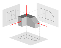
The orthographic projection shows the object as it looks from the front, right, left, top, bottom, or back, and are typically positioned relative to each other according to the rules of either first-angle or third-angle projection. The origin and vector direction of the projectors (also called projection lines) differs, as explained below.

  • In first-angle projection, the projectors originate as if radiated from a viewer's eyeballs and shoot through the 3D object to project a 2D image onto the plane behind it. The 3D object is projected into 2D "paper" space as if you were looking at a radiograph of the object: the top view is under the front view, the right view is at the left of the front view. First-angle projection is the ISO standard and is primarily used in Europe.
  • In third-angle projection, the projectors originate as if radiated from the 3D object itself and shoot away from the 3D object to project a 2D image onto the plane in front of it. The views of the 3D object are like the panels of a box that envelopes the object, and the panels pivot as they open up flat into the plane of the drawing. Thus the left view is placed on the left and the top view on the top; and the features closest to the front of the 3D object will appear closest to the front view in the drawing. Third-angle projection is primarily used in the United States and Canada, where it is the default projection system according to ASME standard ASME Y14.3M.

Until the late 19th century, first-angle projection was the norm in North America as well as Europe;  but circa the 1890s, the meme of third-angle projection spread throughout the North American engineering and manufacturing communities to the point of becoming a widely followed convention,  and it was an ASA standard by the 1950s. Circa World War I, British practice was frequently mixing the use of both projection methods.

As shown above, the determination of what surface constitutes the front, back, top, and bottom varies depending on the projection method used.

Not all views are necessarily used. Generally only as many views are used as are necessary to convey all needed information clearly and economically.The front, top, and right-side views are commonly considered the core group of views included by default, but any combination of views may be used depending on the needs of the particular design. In addition to the 6 principal views (front, back, top, bottom, right side, left side), any auxiliary views or sections may be included as serve the purposes of part definition and its communication. View lines or section lines (lines with arrows marked "A-A", "B-B", etc.) define the direction and location of viewing or sectioning. Sometimes a note tells the reader in which zone(s) of the drawing to find the view or section.

Auxiliary projection 

An auxiliary view is an orthographic view that is projected into any plane other than one of the six principal views. These views are typically used when an object contains some sort of inclined plane. Using the auxiliary view allows for that inclined plane (and any other significant features) to be projected in their true size and shape. The true size and shape of any feature in an engineering drawing can only be known when the Line of Sight (LOS) is perpendicular to the plane being referenced. It is shown like a three-dimensional object.

Isometric projection

The isometric projection show the object from angles in which the scales along each axis of the object are equal. Isometric projection corresponds to rotation of the object by ± 45° about the vertical axis, followed by rotation of approximately ± 35.264° [= arcsin(tan(30°))] about the horizontal axis starting from an orthographic projection view. "Isometric" comes from the Greek for "same measure". One of the things that makes isometric drawings so attractive is the ease with which 60 degree angles can be constructed with only acompass and straightedge.

Isometric projection is a type of axonometric projection. The other two types of axonometric projection are:

  • Dimetric projection
  • Trimetric projection

Oblique projection

An oblique projection is a simple type of graphical projection used for producing pictorial, two-dimensional images of three-dimensional objects:

  • it projects an image by intersecting parallel rays (projectors)
  • from the three-dimensional source object with the drawing surface (projection plan).

In both oblique projection and orthographic projection, parallel lines of the source object produce parallel lines in the projected image.

Perspective

Perspective is an approximate representation on a flat surface, of an image as it is perceived by the eye. The two most characteristic features of perspective are that objects are drawn:

  • Smaller as their distance from the observer increases
  • Foreshortened: the size of an object's dimensions along the line of sight are relatively shorter than dimensions across the line of sight.

Section Views

Projected views (either Auxiliary or Orthographic) which show a cross section of the source object along the specified cut plane. These views are commonly used to show internal features with more clarity than may be available using regular projections or hidden lines. In assembly drawings, hardware components (e.g. nuts, screws, washers) are typically not sectioned.

Scale

Main articles: Architect's scale, Engineer's scale and Metric scale

Plans are usually "scale drawings", meaning that the plans are drawn at specific ratio relative to the actual size of the place or object. Various scales may be used for different drawings in a set. For example, a floor plan may be drawn at 1:50 (1:48 or 1/4"=1'-0") whereas a detailed view may be drawn at 1:25 (1:24 or 1/2"=1'-0"). Site plans are often drawn at 1:200 or 1:100.

Scale is a nuanced subject in the use of engineering drawings. On one hand, it is a general principle of engineering drawings that they are projected using standardized, mathematically certain projection methods and rules. Thus, great effort is put into having an engineering drawing accurately depict size, shape, form, aspect ratios between features, and so on. And yet, on the other hand, there is another general principle of engineering drawing that nearly diametrically opposes all this effort and intent—that is, the principle that users are not to scale the drawing to infer a dimension not labeled. This stern admonition is often repeated on drawings, via a boilerplate note in the title block telling the user, "DO NOT SCALE DRAWING."

The explanation for why these two nearly opposite principles can coexist is as follows. The first principle—that drawings will be made so carefully and accurately—serves the prime goal of why engineering drawing even exists, which is successfully communicating part definition and acceptance criteria—including "what the part should look like if you've made it correctly." The service of this goal is what creates a drawing that one even could scale and get an accurate dimension thereby. And thus the great temptation to do so, when a dimension is wanted but was not labeled. The second principle—that even though scaling the drawing will usually work, one should nevertheless never do it—serves several goals, such as enforcing total clarity regarding who has authority to discern design intent, and preventing erroneous scaling of a drawing that was never drawn to scale to begin with (which is typically labeled "drawing not to scale" or "scale: NTS"). When a user is forbidden from scaling the drawing, s/he must turn instead to the engineer (for the answers that the scaling would seek), and s/he will never erroneously scale something that is inherently unable to be accurately scaled.

But in some ways, the advent of the CAD and MBD era challenges these assumptions that were formed many decades ago. When part definition is defined mathematically via a solid model, the assertion that one cannot interrogate the model—the direct analog of "scaling the drawing"—becomes ridiculous; because when part definition is defined this way, it is not possible for a drawing or model to be "not to scale". A 2D pencil drawing can be inaccurately foreshortened and skewed (and thus not to scale), yet still be a completely valid part definition as long as the labeled dimensions are the only dimensions used, and no scaling of the drawing by the user occurs. This is because what the drawing and labels convey is in reality a symbol of what is wanted, rather than a true replica of it. (For example, a sketch of a hole that is clearly not round still accurately defines the part as having a true round hole, as long as the label says "10mm DIA", because the "DIA" implicitly but objectively tells the user that the skewed drawn circle is a symbolrepresenting a perfect circle.) But if a mathematical model—essentially, a vector graphic—is declared to be the official definition of the part, then any amount of "scaling the drawing" can make sense; there may still be an error in the model, in the sense that what was intended is not depicted (modeled); but there can be no error of the "not to scale" type—because the mathematical vectors and curves are replicas, not symbols, of the part features.

Even in dealing with 2D drawings, the manufacturing world has changed since the days when people paid attention to the scale ratio claimed on the print, or counted on its accuracy. In the past, prints were plotted on a plotter to exact scale ratios, and the user could know that a line on the drawing 15mm long corresponded to a 30mm part dimension because the drawing said "1:2" in the "scale" box of the title block. Today, in the era of ubiquitous desktop printing, where original drawings or scaled prints are often scanned on a scanner and saved as a PDF file, which is then printed at any percent magnification that the user deems handy (such as "fit to paper size"), users have pretty much given up caring what scale ratio is claimed in the "scale" box of the title block. Which, under the rule of "do not scale drawing", never really did that much for them anyway.

Showing dimensions

The required sizes of features are conveyed through use of dimensions. Distances may be indicated with either of two standardized forms of dimension: linear and ordinate.

  • With linear dimensions, two parallel lines, called "extension lines," spaced at the distance between two features, are shown at each of the features. A line perpendicular to the extension lines, called a "dimension line," with arrows at its endpoints, is shown between, and terminating at, the extension lines. The distance is indicated numerically at the midpoint of the dimension line, either adjacent to it, or in a gap provided for it.
  • With ordinate dimensions, one horizontal and one vertical extension line establish an origin for the entire view. The origin is identified with zeroes placed at the ends of these extension lines. Distances along the x- and y-axes to other features are specified using other extension lines, with the distances indicated numerically at their ends.

Sizes of circular features are indicated using either diametral or radial dimensions. Radial dimensions use an "R" followed by the value for the radius; Diametral dimensions use a circle with forward-leaning diagonal line through it, called the diameter symbol, followed by the value for the diameter. A radially-aligned line with arrowhead pointing to the circular feature, called a leader, is used in conjunction with both diametral and radial dimensions. All types of dimensions are typically composed of two parts: the nominal value, which is the "ideal" size of the feature, and the tolerance, which specifies the amount that the value may vary above and below the nominal.

  • Geometric dimensioning and tolerancing is a method of specifying the functional geometry of an object.
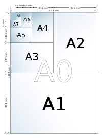
Sizes of drawings

Main article: Paper size

Sizes of drawings typically comply with either of two different standards, ISO (World Standard) or ANSI/ASME Y14 (American), according to the following tables:

 
ISO paper sizes
ISO A Drawing Sizes (mm)
A4 210 X 297
A3 297 X 420
A2 420 X 594
A1 594 X 841
A0 841 X 1189
ANSI/ASME Drawing Sizes (inches)
A 8.5" X 11"
B 11" X 17"
C 17" X 22"
D 22" X 34"
E 34" X 44"
Other U.S. Drawing Sizes
D1 24" X 36"
E1 30" X 42"
H larger still [intracompany standards]
I larger still [intracompany standards]
J larger still [intracompany standards]

The metric drawing sizes correspond to international paper sizes. These developed further refinements in the second half of the twentieth century, when photocopying became cheap. Engineering drawings could be readily doubled (or halved) in size and put on the next larger (or, respectively, smaller) size of paper with no waste of space. And the metric technical pens were chosen in sizes so that one could add detail or drafting changes with a pen width changing by approximately a factor of the square root of 2. A full set of pens would have the following nib sizes: 0.13, 0.18, 0.25, 0.35, 0.5, 0.7, 1.0, 1.5, and 2.0 mm. However, the International Organization for Standardization (ISO) called for four pen widths and set a colour code for each: 0.25 (white), 0.35 (yellow), 0.5 (brown), 0.7 (blue); these nibs produced lines that related to various text character heights and the ISO paper sizes.

All ISO paper sizes have the same aspect ratio, one to the square root of 2, meaning that a document designed for any given size can be enlarged or reduced to any other size and will fit perfectly. Given this ease of changing sizes, it is of course common to copy or print a given document on different sizes of paper, especially within a series, e.g. a drawing on A3 may be enlarged to A2 or reduced to A4.

The U.S. customary "A-size" corresponds to "letter" size, and "B-size" corresponds to "ledger" or "tabloid" size. There were also once British paper sizes, which went by names rather than alphanumeric designations.

American Society of Mechanical Engineers (ASME) Y14.2, Y14.3, and Y14.5 are commonly referenced standards in the U.S.

Technical lettering

Technical lettering is the process of forming letters, numerals, and other characters in technical drawing. It is used to describe, or provide detailed specifications for, an object. With the goals of legibility and uniformity, styles are standardized and lettering ability has little relationship to normal writing ability. Engineering drawings use a Gothic sans-serifscript, formed by a series of short strokes. Lower case letters are rare in most drawings of machines. ISO Lettering templates, designed for use with technical pens and pencils, and to suit ISO paper sizes, produce lettering characters to an international standard. The stroke thickness is related to the character height (for example, 2.5mm high characters would have a stroke thickness - pen nib size - of 0.25mm, 3.5 would use a 0.35mm pen and so forth). The ISO character set (font) has a seriffed one, a barred seven, an open four, six, and nine, and a round topped three, that improves legibility when, for example, an A0 drawing has been reduced to A1 or even A3 (and perhaps enlarged back or reproduced/faxed/ microfilmed &c). When CAD drawings became more popular, especially using US American software, such as AutoCAD, the nearest font to this ISO standard font was Romantic Simplex (RomanS) - a proprietary shx font) with a manually adjusted width factor (over ride) to make it look as near to the ISO lettering for the drawing board. However, with the closed four, and arced six and nine, romans.shx typeface could be difficult to read in reductions. In more recent revisions of software packages, the TrueTypefont ISOCPEUR reliably reproduces the original drawing board lettering stencil style, however, many drawings have switched to the ubiquitous Arial.ttf.

Conventional parts (areas) of an engineering drawing

Title block

The title block (T/B, TB) is an area of the drawing that conveys header-type information about the drawing, such as:

  • Drawing title (hence the name "title block")
  • Drawing number
  • Part number(s)
  • Name of the design activity (corporation, government agency, etc.)
  • Identifying code of the design activity (such as a CAGE code)
  • Address of the design activity (such as city, state/province, country)
  • Measurement units of the drawing (for example, inches, millimeters)
  • Default tolerances for dimension callouts where no tolerance is specified
  • Boilerplate callouts of general specs
  • Intellectual property rights warning

Traditional locations for the title block are the bottom right (most commonly) or the top right or center.

Revisions block

The revisions block (rev block) is a tabulated list of the revisions (versions) of the drawing, documenting the revision control.

Traditional locations for the revisions block are the top right (most commonly) or adjoining the title block in some way.

Next assembly

The next assembly block, often also referred to as "where used" or sometimes "effectivity block", is a list of higher assemblies where the product on the current drawing is used. This block is commonly found adjacent to the title block.

Notes list

The notes list provides notes to the user of the drawing, conveying any information that the callouts within the field of the drawing did not. It may include general notes, flagnotes, or a mixture of both.

Traditional locations for the notes list are anywhere along the edges of the field of the drawing.

General notes

General notes (G/N, GN) apply generally to the contents of the drawing, as opposed to applying only to certain part numbers or certain surfaces or features.

Flagnotes

Flagnotes or flag notes (FL, F/N) are notes that apply only where a flagged callout points, such as to particular surfaces, features, or part numbers. Typically the callout includes a flag icon. Some companies call such notes "delta notes", and the note number is enclosed inside a triangular symbol (similar to capital letter delta, Δ). "FL5" (flagnote 5) and "D5" (delta note 5) are typical ways to abbreviate in ASCII-only contexts.

Field of the drawing

The field of the drawing (F/D, FD) is the main body or main area of the drawing, excluding the title block, rev block, and so on.

List of materials, bill of materials, parts lis

The list of materials (L/M, LM, LoM), bill of materials (B/M, BM, BoM), or parts list (P/L, PL) is a (usually tabular) list of the materials used to make a part, and/or the parts used to make an assembly. It may contain instructions for heat treatment, finishing, and other processes, for each part number. Sometimes such LoMs or PLs are separate documents from the drawing itself.

Traditional locations for the LoM/BoM are above the title block, or in a separate document.

Parameter tabulations

Some drawings call out dimensions with parameter names (that is, variables, such a "A", "B", "C"), then tabulate rows of parameter values for each part number.

Traditional locations for parameter tables, when such tables are used, are floating near the edges of the field of the drawing, either near the title block or elsewhere along the edges of the field.

Views and sections

Each view or section is a separate set of projections, occupying a contiguous portion of the field of the drawing. Usually views and sections are called out with cross-references to specific zones of the field.

Zones

Often a drawing is divided into zones by a grid, with zone labels along the margins, such as A,B,C,D up the sides and 1,2,3,4,5,6 along the top and bottom. Names of zones are thus, for example, A5, D2, or B1. This feature greatly eases discussion of, and reference to, particular areas of the drawing.

Abbreviations and symbols


As in many technical fields, a wide array of abbreviations and symbols have been developed in engineering drawing during the 20th and 21st centuries. For example, cold rolled steel is often abbreviated as CRS, and diameter is often abbreviated as DIA, D, or ⌀.

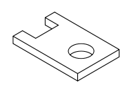
Example of an engineering drawing

 
Example mechanical drawing

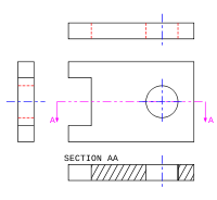
Here is an example of an engineering drawing (an isometric view of the same object is shown above). The different line types are colored for clarity.

  • Black = object line and hatching
  • Red = hidden line
  • Blue = center line of piece or opening
  • Magenta = phantom line or cutting plane line


Graphical projection


Graphical projection
Axonometric projection.svg
Planar[show]
Other[show]
Views[show]
Topics[show]
  •           
                                                                                    
 
                                                     Perspective projection of triangle ABC on plane Π from point S.

Graphical projection is a protocol by which an image of a three-dimensional object is projected onto a planar surface without the aid of numerical calculation, used in technical drawing.[


Overview


                Increasing the focal length and distance of the camera to infinity in a perspective projection results in a parallel projection.

The projection is achieved by the use of imaginary "projectors". The projected, mental image becomes the technician’s vision of the desired, finished picture. By following the protocol the technician may produce the envisioned picture on a planar surface such as drawing paper. The protocols provide a uniform imaging procedure among people trained in technical graphics (mechanical drawing, computer aided design, etc.).

There are two graphical projection categories each with its own protocol:

  • parallel projection
  • perspective projection
  • Isometric projection.

  •  
  • Oblique projection.

  •  
  • Oblique projection.

  •  
  • One-point perspective projection.

Types of projection

 
Several types of graphical projection compared.

Parallel projection

In parallel projection,the lines of sight from the object to the projection plane are parallel to each other. Within parallel projection there is an ancillary category known as "pictorials". Pictorials show an image of an object as viewed from a skew direction in order to reveal all three directions (axes) of space in one picture. Because pictorial projections innately contain this distortion, in the rote, drawing instrument for pictorials, some liberties may be taken for economy of effort and best effect.it is a simultaneous process of viewing the image give pictures

Orthographic projection

The Orthographic projection is derived from the principles of descriptive geometry and is a two-dimensional representation of a three-dimensional object. It is a parallel projection (the lines of projection are parallel both in reality and in the projection plane). It is the projection type of choice for working drawings.

Pictorials

Within parallel projection there is a subcategory known as Pictorials. Pictorials show an image of an object as viewed from a skew direction in order to reveal all three directions (axes) of space in one picture. Parallel projection pictorial instrument drawings are often used to approximate graphical perspective projections, but there is attendant distortion in the approximation. Because pictorial projections inherently have this distortion, in the instrument drawing of pictorials, great liberties may then be taken for economy of effort and best effect. Parallel projection pictorials rely on the technique of axonometric projection ("to measure along axes").

Axonometric projection
 

Axonometric projection is a type of parallel projection used to create a pictorial drawing of an object, where the object is rotated along one or more of its axes relative to the plane of projection.[1]

There are three main types of axonometric projection: isometricdimetric, and trimetric projection.

 
The three axonometric views.
Isometric projection

In isometric pictorials (for protocols see isometric projection), the direction of viewing is such that the three axes of space appear equally foreshortened, and there is a common angle of 60° between them. As the distortion caused by foreshortening is uniform the proportionality of all sides and lengths are preserved, and the axes share a common scale. This enables measurements to be read or taken directly from the drawing.

Dimetric projection

In dimetric pictorials (for protocols see dimetric projection), the direction of viewing is such that two of the three axes of space appear equally foreshortened, of which the attendant scale and angles of presentation are determined according to the angle of viewing; the scale of the third direction (vertical) is determined separately. Approximations are common in dimetric drawings.

Trimetric projection[edit]

In trimetric pictorials (for protocols see trimetric projection), the direction of viewing is such that all of the three axes of space appear unequally foreshortened. The scale along each of the three axes and the angles among them are determined separately as dictated by the angle of viewing. Approximations in Trimetric drawings are common.

Oblique projection

In oblique projections the parallel projection rays are not perpendicular to the viewing plane as with orthographic projection, but strike the projection plane at an angle other than ninety degrees. In both orthographic and oblique projection, parallel lines in space appear parallel on the projected image. Because of its simplicity, oblique projection is used exclusively for pictorial purposes rather than for formal, working drawings. In an oblique pictorial drawing, the displayed angles among the axes as well as the foreshortening factors (scale) are arbitrary. The distortion created thereby is usually attenuated by aligning one plane of the imaged object to be parallel with the plane of projection thereby creating a true shape, full-size image of the chosen plane. Special types of oblique projections are:

Cavalier projection

In cavalier projection (sometimes cavalier perspective or high view point) a point of the object is represented by three coordinates, xy and z. On the drawing, it is represented by only two coordinates, x" and y". On the flat drawing, two axes, x and z on the figure, are perpendicular and the length on these axes are drawn with a 1:1 scale; it is thus similar to the dimetric projections, although it is not an orthographic projection, as the third axis, here y, is drawn in diagonal, making an arbitrary angle with the x" axis, usually 30 or 45°. The length of the third axis is not scaled.

Cabinet projection

The term cabinet projection (sometimes cabinet perspective) stems from its use in illustrations by the furniture industry.[citation needed] Like cavalier perspective, one face of the projected object is parallel to the viewing plane, and the third axis is projected as going off in an angle (typical 30° or 45° or arctan(2)=63.4°). Unlike cavalier projection, where the third axis keeps its length, with cabinet projection the length of the receding lines is cut in half.

Perspective projection

 
Axonometric projection of a scheme displaying the relevant elements of a vertical picture planeperspective. The standing point (P.S.) is located on the ground plane π, and the point of view (P.V.) is right above it. P.P. is its projection on the picture plane α. L.O. and L.T. are the horizon and the ground lines (linea d'orizzonte and linea di terra). The bold lines sand q lie on π, and intercept α in Ts and Tq respectively. The parallel lines through P.V. (in red) intercept L.O. in the vanishing points Fs and Fq: thus one can draw the projections s' and q', and hence also their intersection R', the projection of R.
 
Perspective of a geometric solid using two vanishing points. In this case, the map of the solid (orthogonal projection) is drawn below the perspective, as if bending the ground plane.
Main article: Perspective (graphical)

Perspective projection is a linear projection where three dimensional objects are projected on a picture plane. This has the effect that distant objects appear smaller than nearer objects.

It also means that lines which are parallel in nature (that is, meet at the point at infinity) appear to intersect in the projected image, for example if railways are pictured with perspective projection, they appear to converge towards a single point, called vanishing point. Photographic lenses and the human eye work in the same way, therefore perspective projection looks most realistic.[2] Perspective projection is usually categorized into one-point, two-point and three-point perspective, depending on the orientation of the projection plane towards the axes of the depicted object.[3]

Graphical projection methods rely on the duality between lines and points, whereby two straight lines determine a point while two points determine a straight line. The orthogonal projection of the eye point onto the picture plane is called the principal vanishing point (P.P. in the scheme on the left, from the Italian term punto principale, coined during the renaissance).[4]

Two relevant points of a line are:

  • its intersection with the picture plane, and
  • its vanishing point, found at the intersection between the parallel line from the eye point and the picture plane.

The principal vanishing point is the vanishing point of all horizontal lines perpendicular to the picture plane. The vanishing points of all horizontal lines lie on the horizon line, obviously. If, as is often the case, the picture plane is vertical, all vertical lines are drawn vertically, and have no finite vanishing point on the picture plane. Various graphical methods can be easily envisaged for projecting geometrical scenes. For example, lines traced from the eye point at 45° to the picture plane intersect the latter along a circle whose radius is the distance of the eye point from the plane, thus tracing that circle aids the construction of all the vanishing points of 45° lines; in particular, the intersection of that circle with the horizon line consists of two distance points. They are useful for drawing chessboard floors which, in turn, serve for locating the base of objects on the scene. In the perspective of a geometric solid on the right, after choosing the principal vanishing point —which determines the horizon line— the 45° vanishing point on the left side of the drawing completes the characterization of the (equally distant) point of view. Two lines are drawn from the orthogonal projection of each vertex, one at 45° and one at 90° to the picture plane. After intersecting the ground line, those lines go toward the distance point (for 45°) or the principal point (for 90°). Their new intersection locates the projection of the map. Natural heights are measured above the ground line and then projected in the same way until they meet the vertical from the map.

 Drawing layout and Lettering

Layout of a drawing sheet 
Every drawing sheet is to follow a particular layout.  As a standard practice sufficient margins are to be provided on all sides of the drawingsheet.  The drawing sheet should have drawing space and title page.  A typical layout of a drawing sheet is shown in the figure below:

Figure 1. A typical layout of a drawing sheet.

  • Borders – A minimum of 10 mm space left all around in between  the trimmed edges of the sheet.
  • Filing margin – Minimum 20 mm space left on the left hand side with border included. This provided for taking perforations .
  • Grid reference system – This is provided on all sizes of industrial drawing sheets for easy location of drawing within the frame.  The length and the width of the frames are divided into even number of divisions and labeled using numerals or capital letters.  Number of divisions for a particular sheet depends on complexity of the drawing. The grids along the horizontal edges  are labeled in numerals where as grids  along vertical edges are labeled using capital letters. The length of each grids can be between 25 mm and 75 mm.  Numbering and lettering start from the corner of the sheet opposite to the title box and are repeated on the opposite sides. they are written upright. Repetition of letters or numbers like AA, BB, etc., if they exceed that of the alphabets. For first year engineering students grid references need not be followed.
  • Title box – An important feature on every drawing sheet.  This  is located at the bottom right hand corner of every sheet and provides the technical and administrative details of the drawing.  The title box is divided into two zones
    1. Identification zone : In this zone the details like the identification number or part number, Title of the drawing, legal owner of the drawing, etc. are to be mentioned.
    2. Additional information zone : Here indicative items lime symbols indicting the system of projection,  scale used, etc., the technical items lime method of surface texture, tolerances, etc., and other administrative items are  to be mentioned.

Layout of the title box recommended for Engineering Drawing Course
The title box shown in figure 2  can be used for  the engineering Drawing Course.

Figure 2. A typical title box recommended for Engineering students.

Lettering 
Lettering is used for writing of titles, sub-titles, dimensions, scales and other details on a drawing. Typical lettering features  used for engineering drawing is shown in figure 3. The following rules are to be followed in lettering. The letter  sizes generally recommended for various items are shown in Table 1.

  • Essential features of lettering – legibility, uniformity, ease, rapidity, and suitability for microfilming/photocopying/any other photographic processes
  • No ornamental and embellishing style of letter
  • Plain letters and numerals which are clearly distinguishable from each other in order to avoid any confusion even in case of slight mutilations

The Indian standard followed for lettering is  BIS: 9609

  • Single stroke lettering for use in engineering drawing – width of the stem of the letters and numerals will be uniformly thick equal to thickness of lines produced by the tip of the pencil.
  • Single stroke does not mean – entire letter written without lifting the pencil/pen

Lettering types generally used for creating a drawing are

  • Lettering A – Height of the capital letter is divided into 14 equal parts
  • Lettering B – Height of the capital letter is divided into 10 equal parts

Table 2  and Table 3 indicates the specifications for Type A and Type B letters.


Figure 3. Typical lettering  features.


Heights of Letters and Numerals

  1. Height of the capital letters is equal to the height of the numerals used in dimensioning
  2. Height of letters and numerals – different for different purposes

Table 1 The letter  sizes recommended for various items

Table 2. Specifications of A -Type Lettering                        


Table 3. Specifications of B -Type Lettering

How to begin your drawing? 
To start with the preparation of a drawing the procedure mentioned below may be followed:

  • Clean the drawing board and all the drawing instruments using duster.
  • Fix the drawing sheet on the drawing board.
  • Fix the mini-drafter in a convenient position.
  • Draw border lines using HB pencil..
  • Complete the title box using HB pencil .
  • Plan spacing of drawings b/n two problems/views beforehand.
  • Print the problem number on the left top and then commence the drawing work.

Keeping the drawing clean is  a must

  • Never sharpen pencils over drawing.
  • Clean pencil point with a soft cloth after sharpening.
  • Keep drawing instruments clean.
  • Rest hands on drawing instruments as much as possible – to avoid smearing the graphite on the drawing.
  • When darkening lines – try to work from the top of the drawing to the bottom, and from left to the right across the drawing.
  • Use brush to remove eraser particles. Never use hands.
  • Always use appropriate drawing pencils.

 Lines and Dimensioning

Lines 
Lines is one important aspect of technical drawing.  Lines are always used to construct meaningful drawings. Various types of lines are used to construct drawing, each line used in some specific sense.  Lines are drawn following standard conventions mentioned in BIS (SP46:2003). A line may be curved, straight, continuous, segmented. It may be drawn as thin or thick. A few basic types of lines widely used in drawings are shown in Table 1.  

Table 1. Types of letters used in engineering drawing.


Line Strokes 
Line strokes refer to the directions of drawing straight and curved lines. The standards for lines is  given in  BIS : SP-46,  2003 
Vertical and inclined lines are drawn from top to bottom, horizontal lines are drawn from left to right. Curved lines are drawn from left to right or top to bottom. The direction of strokes are illustrated in figure 1.

Figure 1. The line strokes  for drawing straight and curved lines.

Conventions used in lines

  • International systems of units (SI) – which is based on the meter.
  • Millimeter (mm) - The common SI unit of measure on engineering drawing.
  • Individual identification of linear units is not required if all dimensions on a drawing are in the same unit (mm).
  • The drawing should contain a note: ALL DIMENSIONS ARE IN MM. (Bottom left corner outside the title box)

Typical figures showing various lines used in the construction of engineering drawing is shown in figure 2.

  Figure 2  Typical figure showing various lines used engineering drawing

A typical use of various lines in an engineering drawing is shown in figure below:


Dimensioning 
The size and other details of the object essential for its construction and function, using lines, numerals, symbols, notes, etc are required to be indicated in a drawing by proper dimensioning. These dimensions indicated should be those that are essential for the production, inspection and functioning of the object and should be mistaken as those that are required to make the drawing of an object.  The dimensions are written either above the dimension lines or inserted at the middle by breaking the dimension lines.

Normally two types of dimensioning system exist. i.e. Aligned system and the unidirectional system.These are shown in figure 3.

In the aligned system the dimensions are placed perpendicular to the dimension line in such a way that it may be read from bottom edge or right hand edge of the drawing sheet. The horizontal and inclined dimension can be read from the bottom where as all the vertical dimensions can be read from the right hand side of the drawing sheet. 
In the unidirectional system, the dimensions are so oriented such that they can be read from the bottom of the drawing.


Figure 3. The aligned system and unidirectional system of dimensioning.


Rules to be followed for dimensioning. Refer figure 4.

  • Each feature is dimensioned and positioned only once.
  • Each feature is dimensioned and positioned where its shape shows.
  • Size dimensions – give the size of the component.
  • Every solid has three dimensions, each of the geometric shapes making up the object must have its height, width, and depth indicated in the dimensioning.


Figure 4. typical dimension lines


Dimensioning consists of the following:

  • A  thin, solid line that shows the extent and direction of a dimension.  Dimension lines are broken for insertion of the dimension numbers
  • Should be placed at least 10 mm away from the outline and all
  • other parallel dimensions should be at least 6 mm apart, or more, if space permits

The important elements of dimensioning consists of extension lines, leader line, arrows and dimensions.

Extension line – a thin, solid line perpendicular to a dimension line, indicating which feature is associated with the dimension. There should be a visible gap of 1.5 mm between the feature’s corners and the end of the extension line.Figure 5 shows extension lines.
Leader line 
A thin, solid line used to indicate the feature with which a dimension, note, or symbol is associated.   Generally this is  a straight line drawn at an angle that is neither horizontal nor vertical.  Leader line is terminated with an arrow touching the part or detail.  On the end opposite the arrow, the leader line will have a short, horizontal shoulder.  Text is extended from this shoulder such that the text height is centered  with the shoulder line

Figure 5. showing extension lines

  • Arrows –  3 mm wide and should be 1/3rd as wide as they are long - symbols placed at the end of dimension lines to  show the limits of the dimension.  Arrows are uniform in size and style, regardless of the size of the drawing.Various types of arrows used for dimensioning is shown in figure 6.

Figure 6.Various types of arrows used for dimensioning


The specification of dimension lines are shown in figure 7.

Figure 7 showing the specification of dimension lines.  

Dimensioning of angles: The normal convention for dimensioning of angles are illustrated in figure 8.


Figure 8  conventions used for dimensioning angles.


Few examples during dimensioning of solids are shown below:

  • Prism –    This is the most common shape and requires three dimensions. Two dimensions shown on the  principal view and  the third dimension on the other view.

  • Cylinder – Cylinder is the second most common shape. It requires  two dimensions: diameter and length, both shown preferably on the rectangular view.

  • Cone – requires two dimensions – diameter of the base and altitude  on the same view and length. Both shown on the rectangular view is preferred.


  • Right pyramids – requires three dimensions – dimensions  of the base and altitude.

  • Spheres – requires   only one dimension. i.e. diameter. However in case of extra features, those dimensions are required to be provided.


RULES OF DIMENSIONING

  1. Between any two extension lines, there must be one and only one dimension line bearing one dimension.
  2. As far as possible, all the dimensions should be placed outside the views. Inside dimensions are preferred only if they are clearer and more easily readable.
  3. All the dimensions on a drawing must be shown using either Aligned System or Unidirectional System. In no case should, the two systems be mixed on the same drawing.
  4. The same unit of length should be used for all the dimensions on a drawing. The unit should not be written after each dimension, but a note mentioning the unit should be placed below the drawing.
  5. Dimension lines should not cross each other. Dimension lines should also not cross any other lines of the object.
  6. All dimensions must be given.
  7. Each dimension should be given only once. No dimension should be redundant.
  8. Do not use an outline or a centre line as a dimension line. A centre line may be extended to serve as an extension line.
  9. Avoid dimensioning hidden lines.
    1. Chain dimensioning (Continuous dimensioning) All the dimensions are aligned in such a way that an arrowhead of one dimension touches tip-to-tip the arrowhead of the adjacent dimension. The overall dimension is placed outside the other smaller dimensions.
    2. Parallel dimensioning (Progressive dimensioning) All the dimensions are shown from a common reference line. Obviously, all these dimensions share a common extension line. This method is adopted when dimensions have to be established from a particular datum surface
    3. Combined dimensioning.  When both the methods, i.e., chain dimensioning and parallel dimensioning are used on the same drawing, the method of dimensioning is called combined dimensioning. 
  10. For dimensions in series, adopt any one of the following ways.


Geometrical Constructions: Part-1

Geometric Construction

Drawing consists of construction of primitive geometric forms viz.  points, lines and planes that serve a the building blocks for more complicated geometric shapes and defining the position of object in space.

The use of lines for obtaining the drawing of planes is shown in figure 1.

Figure 1 illustrates various planes generally encountered


Solids are obtained by combination of planes. Plane surfaces of  simple solids are shown in figure 2.


Figure 2 surfaces of few simples solids .  

In addition curved surfaces also exists. Figure 3 shows some of  solids having curved surfaces.


Figure 3. Solids having curved surfaces.

Primitive geometric forms
The shapes of objects are formed from primitive geometric forms . These are

  1. Point
  1. Line
  2. Plane
  3. Solid
  4. Doubly curved surface and object
  5. Warped surface

  The basic 2-D geometric primitives, from which other more complex geometric forms are derived.

  • Points,
  • Lines,
  • Circles, and 
  • Arcs

Point

A point is a theoretical location that has neither width, height, nor depth and  describes exact location in space. A point is represented in technical drawing as a small cross made of dashes that are approximately 3 mm long. As shown in figure 4, a point is used to mark the locations of  centers and loci, the intersection ends, middle of entities


Figure 4. shows the various use of points.

Line

A line is a geometric primitive that has length and direction, but no thickness. Lines may be straight, curved or a combination of these. As shown in figure 5, lines have few important relationship or conditions, such as parallel, intersecting, and tangent.  Lines can be of specific length or non-specific length. A Ray is a sStraight line that extends to infinity from a specified point.


Figure 5. Relationship of one line to another line or arc


Bisecting a line

The procedure of bisecting a given line AB is illustrated in figure 6. 
With A as centre and radius equal to higher than half AB, draw two arcs. With B as centre and with the same radius draw another arc intersecting the preious arcs. The line joining the intersection points is the perpendicular bisector of the line AB.


Figure 6. Illustrates the method of bisecting a line

Dividing a line into equal parts

The method of dividing a line MO  into equal number of parts is illustrated in figure 7.

  • Draw a line MO at any convenient angle (preferably an acute angle) from point M.
  • From M and along MO, cut off with a divider equal divisions (say three) of any convenient length.
  • Draw a line joining ON.
  • Draw lines parallel to MO through the remaining points on line MO.
The intersection of these lines with line MN will divide the line into (three) equal parts.


Figure 7. Dividing a line in to equal number of parts.


Planar tangent condition exists when two geometric forms meet at a single point and do not intersect. This is self explanatory from figure 8.


Figure 8. Illustrates the existence of  planar tangent condition.

Locating tangent points on circle and arcs

The method of locating tangent points on circle and arcs as well as thhe common tangent to two circles  are shown in figure 9(a) and (b) .

Figure 9. Locating the tangent points to arcs or circles.

Drawing an arc tangent to a given point on the line 
The steps  for drawing the arc tangent to a given point on a line is shown in figure 10.

  1. Given line AB and tangent point T. Construct a line perpendicular to line AB and through point T.
  2. Locate the center of the arc by making the radius on the perpendicular line. Put the point of the compass at the center of the arc, set the compass for the radius of the arc, and draw the arc which will be tangent to the line through the point T.


Figure 10. Drawing an arc tangent to the a given point on a line.


Drawing an arc, tangent to two lines

The steps used to drawn an arc tangent to two lines  is illustrated in figure 11.

Figure 11. illustrates the method of drawing an arc tangent to two lines.


Drawing an arc, tangent to a  line and an arc

Figure 12 shows the steps in drawing an arc tangent to a line and an arc that  (a) that do not intersect  and  (b) that intersect each other.


Figure 12 Drawing an arc tangent to a line and an arc


Geometric construction: Part-2

Construction of Regular Polygon of given length AB

To construct a regular polygon with length of edge AB us shown in figure 1.

Figure 1. Construction of a regular polygon with a given length of edge.

  • Draw a line of length AB.  With A as centre and radius AB, draw a semicircle.
  • With the divider, divide the semicircle into the number of sides  (example of number of side 7 is shown in figure 1) of the polygon.
  • Draw a line joining A with the second division-point 2.
  • The perpendicular bisectors of A2 and AB meet at O. Draw a circle with centre O and radius OA.
  • With length A2, mark points F, E, D & C on the circumferences starting from 2 (Inscribe circle method)
  • With centre B and radius AB draw an arc cutting the line A6 produced at C.  Repeat this for other points D, E & F (Arc method)

General method of drawing any polygon

A more general method of drawing any polygon with a given length of edge is shown in figure 2.

  • Draw AB = given length of polygon
  • At B, Draw BP perpendicular & = AB
  • Draw Straight line AP
  • With center B and radius AB, draw arc AP.
  • The perpendicular bisector of AB meets the line AP and arc AP in 4 and 6 respectively.
  • Draw circles with centers as 4, 5,&6 and radii as 4B, 5B, & 6B and inscribe a square, pentagon, & hexagon in the respective circles.
  • Mark point 7, 8, etc  with 6-7,7-8,etc. = 4-5 to get the centers of circles of heptagon and octagon, etc.

Figure 2 Drawing any polygon with a given length of edge

Inscribe a circle inside a regular polygon

The method of inscribing a circle inside a regular polygon is illustrated in figure 3.

  1. Bisect any two adjacent internal angles of the polygon.
  2. From the intersection of these lines, draw a perpendicular to any one side of the polygon (say OP).
  3. With OP as radius, draw the circle with O as cente

Figure 3 Inscribing a circle inside a regular polygon

Inscribe a regular polygon of any number of sides (say n = 5), in a circle

Figure 4 shows the method of inscribing a regular polygon of any number of sides.

  • Draw the circle with diameter AB.
  • Divide AB in to “n” equal parts
  • Number them.
  • With center A & B and radius AB, draw arcs to intersect at P.
  • Draw line P2 and produce it to meet the circle at C.
  • AC is the length of the side of the polygon.

Figure 4 Inscribing a regular polygon of any number of sides.

To draw a circle to touch a given line, and a given circle at a given point on it.

The method is illustrated in figure 5.

  • Given: Line AB, circle with centre C and point P on the circle.
  • From P, draw a tangent to the circle intersecting AB at D.
  • Draw bisector of  angle PDB to intersect the line through C and P at O.
  • With center O and radius OP, draw the required circle.


Figure 5.  shows the method of drawing a circle to touch a given line and a given circle at a particular point. 


Inside a regular polygon, draw the same number of equal circles as the side of the polygon,each circle touching one side of the polygon and two of the other circles

The technique is shown in figure 6

  • Draw bisectors of all the angles of the polygon, meeting at O, thus dividing the polygon into the same number of triangles.
  • In each triangle inscribe a circle.

Figure 6.  Drawing the same number of equal circles, in a given polygon , as the side of the polygon

Figure 7  shows the technique for drawing the same number of equal circles as the side of the polygon inside a regular polygon, each circle touching two adjacent sides of the polygon and two of the other circles.

  • Draw the perpendicular bisectors of the sides of the polygon to obtain same number of  quadrilaterals as the  number of sides of the polygon.
  • Inscribe a circle inside each quadrilateral.

Figure 7. drawing the same number of equal circles as the side of the polygon inside a regular polygon

Figure 8 shows the method of drawing a circle touching three lines inclined to each other but not forming a triangle.

  • Let AB, BC, and AD be the lines.
  • Draw bisectors  of the two angles, intersecting at O.
  • From O draw a perpendicular to any one line intersecting it at P.
  • With O as center and OP as radius draw the desired circle.


Figure 9 shows the method of drawing  outside a regular polygon, the same number of equal circles as the sides of the polygon, each circle touching one side of the polygon and two of the other circles.

  • Draw bisectors of two adjacent angles and produce them outside the polygon.
  • Draw a circle touching the extended bisectors and the side AB (in this case) and repeat the same for other sides.

Figure 9 shows the method of drawing  outside a regular polygon, the same number of equal circles as the sides of the polygon,


Scales

Scales

There is a wide variation in sizes for engineering objects. Some are very large (eg. Aero planes, rockets, etc) Some are vey small ( wrist watch, MEMs components) 
There is a need to reduce or enlarge while drawing the objects on paper. Some objects can be drawn to their actual size. The proportion by which the drawing of aan object is enlarged or reduced is called the scale of the drawing.

Definition
A scale is defined as the ratio of the linear dimensions of the object as  represented in a drawing to the actual dimensions of the same.

  • Drawings drawn with the same size as the objects are called full sized drawing.
  • It is not convenient, always, to draw drawings of the object to its actual size. e.g. Buildings,
  • Heavy machines, Bridges, Watches, Electronic devices etc.
  • Hence scales are used to prepare drawing at
  • Full size
  • Reduced size 
  • Enlarged size

BIS Recommended Scales are shown in table 1.

Table 1. The common scales recommended.

Intermediate scales can be used in exceptional cases where recommended scales can not be applied for functional reasons.

Types of Scale :-
Engineers Scale :  The relation between the dimension on the drawing and the actual dimension of the object is mentioned numerically  (like 10 mm = 15 m).

Graphical Scale:  Scale is drawn on the drawing itself. This takes care of the shrinkage of the engineer’s scale when the drawing becomes old.

Types of Graphical Scale :-

  • Plain Scale
  • Diagonal Scale
  • Vernier Scale
  • Comparative scale
  • Scale of chords

Representative fraction (R.F.) :-

When a 1 cm long line in a drawing represents 1 meter length of the object

Length of scale  = RF x Maximum distance to be represented

Plain scale :-

  • A plain scale is  used to indicate the distance in a unit and its nest subdivision.
  • A plain scale consists of a line divided into suitable number of equal units. The first unit is subdivided into smaller parts.
  • The zero should be placed at the end of the 1st main unit.
  • From the zero mark, the units should be numbered to the right and the sub-divisions to the left.
  • The units and the subdivisions should be labeled clearly.
  • The R.F. should be mentioned below the scale.


Construct a plain scale of RF = 1:4, to show centimeters and long enough to measure up to 5 decimeters.

  • R.F. = ¼
  • Length of the scale  = R.F. × max. length = ¼  × 5 dm  = 12.5 cm.
  • Draw a line 12.5 cm long and divide it in to 5 equal divisions, each representing 1 dm.
  • Mark 0 at the end of the first division and 1, 2, 3 and 4 at the end of each subsequent division to its right.
  • Divide the first division into 10 equal sub-divisions, each representing 1 cm.
  • Mark cm to the left of 0 as shown.
  • Draw the scale as a rectangle of small width (about 3 mm) instead of only a line.
  • Draw the division lines showing decimeters throughout the width of the scale.
  • Draw thick and dark horizontal lines in the middle of all alternate divisions and sub-divisions.
  • Below the scale, print DECIMETERS on the right hand side, CENTIMERTERS on the left hand side, and R.F. in the middle.


Diagonal Scale :-

  • Through Diagonal scale, measurements can be up to second decimal places (e.g.  4.35).
  • Are used to measure distances in a unit and its immediate two subdivisions; e.g. dm, cm & mm, or yard, foot & inch.
  • Diagonal scale can measure more accurately than the plain scale.

Diagonal scale…..Concept

  • At end B of line AB, draw a perpendicular.
  • Step-off ten equal divisions of any length along the perpendicular starting from B and ending at C.
  • Number the division points 9,8,7,…..1.
  • Join A with C.
  • Through the points 1, 2, 3, etc., draw lines parallel to AB and cutting AC at 1΄, 2΄, 3΄, etc.
  • Since the triangles are similar; 1΄1 = 0.1 AB, 2΄2 = 0.2AB, …. 9΄9 = 0.9AB.
  • Gives divisions of a given short line AB in multiples of 1/10 its length, e.g. 0.1AB, 0.2AB, 0.3AB, etc.


Construct a Diagonal scale of RF = 3:200  showing meters, decimeters and centimeters. The scale should measure up to 6 meters. Show a distance of 4.56 meters

  • Length of the scale  =  (3/200) x 6 m  = 9 cm
  • Draw a line AB = 9 cm . Divide it in to 6 equal parts.
  • Divide the first part A0 into 10 equal divisions.
  • At A draw a perpendicular and step-off along it 10 equal divisions, ending at D.

Diagonal Scale


  • Complete the rectangle ABCD.
  • Draw perpendiculars at meter-divisions i.e. 1, 2, 3, and 4.
  • Draw horizontal lines through the division points on AD. Join D with the end of the first division along A0 (i.e. 9).
  • Through the remaining points i.e. 8, 7, 6, … draw lines // to D9.
  • PQ = 4.56 meters

Vernier Scale


  • Similar to Diagonal scale, Vernier scale is used for measuring up to second decimal.
  • A Vernier scale consists of (i) a main scale  and (ii) a vernier.
  • The main scale is a plain scale fully divided in to minor divisions. A subdivision on the mail scale is called the  main scale division (MSD) .
  • The graduations on the vernier are derived from those on the primary scale. A subdivision on the verscale is called the vernier scale division (VSD).

Least Count  (LC)  is the minimum length that can be measured precisely by a given vernier scale. This can be determined by the following expression:
LC = MSD – VSD     ( if MSD > VSD) 
LC = VSD  – MSD     ( if VSD > MSD) 
The LC is mentioned as a fraction of the MSD. 
If the MSD of a scale represents 1 mm and LC  is 0.1 mm,

LC = 0.1 mm  = (1/10) MSD

  1. Assume MSD > VSD   
    LC = MSD –VSD 
    1/10 MSD  = MSD –VSD 
    i.e.,  VSD  = MSD – 1/10 MSD 
    10 VSD  = 9 MSD 
    i.e., Length of VSD  = 9 MSD. 

This length must be divided in to 10 equal parts so that LC = 0.1 mm

  1. Assume VSD > MSD 
    LC = VSD – MSD 
    1/10 MSD = VSD – MSD 
    i.e.,  VSD = 1/10 MSD + MSD 
    10 VSD = 11 MSD 
    This length is to be divided in to 20 equal parts so that LC = 0.1 mm

Backward Vernier scale


  • Length A0 represents 10 cm and is divided in to 10 equal parts each representing 1 cm.
  • B0 = 11 (i.e. 10+1) such equal parts =  11 cm.
  • Divide B0 into 10 equal divisions. Each division of B0 will be equal to 11/10 = 1.1 cm or 11 mm.
  • Difference between 1 part of A0 and one part of B0 = 1.1 cm -1.0 cm = 0.1cm or 1 mm.


Question: Draw a Vernier scale of R.F. = 1/25 to read up to 4 meters. On it show lengths 2.39 m and 0.91 m


  • Length of Scale = (1/25) × (4 × 100) = 16 cm
  • Draw a 16 cm long line and divide it into 4 equal parts. Each part is 1 meter.  Divide each of these parts in to 10 equal parts to show decimeter (10 cm).
  • Take 11 parts of dm length and divide it in to 10 equal parts. Each of these parts will show a length of 1.1 dm or 11 cm.
  • To measure 2.39 m, place one leg of the divider at on 99 cm mark and other leg at B on 1.4 mark.  (0.99 + 1.4 = 2.39).
  • To measure 0.91 m, place the divider at C and D (0.8 +0.11 = 0.91).

Comparative Scales

  • Comparative Scale consists of two scales of the same RF, but graduated to read different unit,constructed separately or one above the other.
  • Used to compare distances expressed in different systems of unit e.g. kilometers and miles,
  • centimeters and inches.The two scales may be plain scales or diagonal scales or Vernier scales.  

1 Mile = 8 fur. = 1760 yd = 5280 ft

Construct a plain comparative Scales of RF = 1/624000 to read up to 50 kms and 40 miles. 
On these show the kilometer equivalent to 18 miles


Draw a 4 in. line AC and construct a plain scale to represent mile and 8cm line AB and construct the kilometer scale below the mile scale. 
On the mile scale, determine the distance equal to 18 miles (PQ) 
Mark P’Q’ = PQ on the kilometer scale such that P’ will coincide with the appropriate main division.  Find the length represented by P’Q’.  
P’Q’ = 29 km.           (1Mile = 1.60934 km)


Scale of chords

Scale of chords is used to measure angles when a protractor is not available, by comparing the angles subtended by chords of an arc at the centre of the arc. 
Draw a line AO of any suitable length. 
At O, erect a perpendicular OB such that OB – OA 
With O as centre, draw an arc AB 
Divide the arc in to 9 equal parts  by the following method.

  1. On arc AB, mark two arcs with centers A and B and radius – AO. By this the arc AB is divided in to three equal parts.
  2. By trial and error method, divide each of these three parts in to three equal subdivisions.

The total length of AB is now divided in to 9  equal parts. Number the divisions as 10, 20, 30, 40 ,etc. 
Transfer all the divisions on the arc to th line AO by drawing arcs with A as a centre and radii equal to the chords A-10, 10-20, 20-30, …. AB. 
Construct the linear degree scale by drawing the rectangles below AC.  Mark the divisions in the rectangle with zero below A and number the divisions subsequently as 10o, 20o, 30o, 40o, ….., 90o


 Engineering curves: Ellipse

Conic curves (conics) 
Curves formed by the intersection of a plane with a right circular cone. e.g. Parabola, hyperbola and ellipse. Right circular cone is a cone that has a circular base and the axis is inclined at 900 to  the base and passes through  the center of    the base.Conic sections are always "smooth". More precisely, they never contain any inflection points.  This is important for many applications, such as aerodynamics, civil engineering, mechanical engineering, etc.Figure 1. Shows a right cone and the various conic curves that can be obtained from a cone by sectioning the cone at various conditions.


Figure 1. Shows a right cone and the various conic curves that can be obtained from a cone by sectioning the cone at various conditions.

Conic

Conic is defined as the locus of a point moving in a plane such that the ratio of its distance from a fixed point and a fixed straight line is always constant.

  • Fixed point  is called Focus
  • Fixed line is called Directrix

This is illustrated in figure 2.


Figure 2.  illustrates the directrices and foci of a conic curve.


When eccentricity 
<  1   Ellipse 
=1    Parabola 
> 1    Hyperbola     

 eg. when e=1/2, the curve is an  Ellipse, when e=1, it is a parabola and when e=2, it is a hyperbola.  Figure 3 shows the ellipse, parabola and hyperbola.


Figure 3 shows the relationship of eccentricity with different conic curves.

Ellipse

Referring to figure 4, an ellipse can be defined in the following ways.

  • An ellipse is obtained when a sectio plane, inclined to the axis of the cone , cuts all the generators of the cone.
  • An ellipse is the set of all points in a plane for which the sum of the distances from the two fixed points (the foci) in the plane is constant
  • An ellipse is also defined  as a curve traced by a point, moving in a plane such that the sum of its distances from two fixed points is always the same.

Construction of Ellipse

  1. When the  distance of the directrix from the focus and eccentricity is given.
  2. Major axis and minor axis is given.
  3. Arc of circle method
  4. Concetric circle method
  5. Oblong method
  6. Loop of the thread method


Figure 4. illustrating an ellipse.

Focus-Directrix or Eccentricity Method 
Given : the distance of focus from the directrix and  eccentricity 
Figure 5. shows the method of drawing an ellipse if the distance of focus from the directrix is 80 mm and the eccentricity is 3/4.

  1. Draw the directrix AB and axis CC’
  2. Mark F on CC’ such that CF = 80 mm.
  3. Divide CF into 7 equal parts and mark V at the fourth division from C. Now, e = FV/ CV = 3/4.
  4. At V, erect a perpendicular VB = VF. Join CB. Through F, draw a line at 45° to meet CB produced at D. Through D, drop a perpendicular DV’ on CC’. Mark O at the midpoint of V– V’.

Figure 5. drawing an ellipse if the distance of focus from the directrix and the eccentricity is given                 

5.With F as a centre and radius = 1–1’, cut two arcs on the perpendicular through 1 to locate P1 and P1’. Similarly, with F as centre and radii = 2–2’, 3–3’, etc., cut arcs on the corresponding perpendiculars to locate P2 and P2’, P3 and P3’, etc. Also, cut similar arcs on the perpendicular through O to locate V1 and V1’.

6.Draw a smooth closed curve passing through V, P1, P/2, P/3, …, V1, …, V’, …, V1’, … P/3’, P/2’, P1’.

7.Mark F’ on CC’ such that V’ F’ = VF.

An ellipse is also the set of all points in a plane for which the sum of the distances from the two fixed points (the foci) in the plane is constant.This is clear from figure 6.


Figure 6.Another definition of ellipse

Arcs of Circle Method 
The arc of circle method of drawing an ellipse is generally used  when (i) the major axies and minor axis are known, and (ii) the major axis and the distance between the foci are know.   Themethod of drawing the ellipse by the arcs of circle method is as follows and is shown in figure 7.

Draw AB & CD perpendicular to each other as the major diameter minor diameter respectively. 
With centre as C or D, and half the major diameter as radius draw arcs to intersect the major diameter to obtain the foci at X and Y. 
Mark a number of points along line segment XY and number them. Points need not be equidistant. 
Set the compass to radius B1 and  draw two arcs, with Y as center.  Set the compass to radius A1, and draw two arcs with X as center. Intersection points of the two arcs are points on the ellipse. Repeat this step for all the remaining points. Use the French curve to connect the points, thus drawing the ellipse.


Figure 7. Drawing an ellipse by arcs of circle method.

Constructing an Ellipse (Concentric Circle Method)

Concentric circle method is  is used when the  major axis and minor axis of the ellipse iis given. This method is illustrated in figure 8 and  discussed below:

  • With center C, draw two concentric circles with diameters equal to major and minor diameters of the ellipse.  Draw the major and minor diameters. 
  • Construct a  line AB at any angle through C.  Mark points D and E where the line intersects the smaller circle.
  • From points A and B, draw lines parallel to the minor diameter. Draw lines parallel to the major diameter through D & E. 
  • The intersection of the lines from A and D is point F, and from B and E is point G.  Points F & G lies on the ellipse.
  • Extend lines FD & BG and lines AF and GE to obtain two more points in the other quadrants.
  • Repeat steps 2-6 to create more points in each quadrant and then draw a smooth curve through the points.
  • With center C, draw two concentric circles with diameters equal to major and minor diameters of the ellipse.  Draw the major and minor diameters. 

Figure 8. Concentric circle method of drawing ellipse


Drawing Tangent and Normal to any conic

When a tangent at any point on the curve (P) is produced to meet the directrix, the line joining the focus with this meeting point (FT) will be at right angle to the line joining the focus with the point of contact (PF). 
The normal to the curve at any point is perpendicular to the tangent at that point.


  Figure 9. The method of drawing tangent and normal to any conic section at a particular point.    


Parabola

Parabola

A parabola is obtained when a section plane, parallel to one of the generators cuts the cone. This is illustrated in figure 1.

Figure 1.  Obtaining a parabola from a cone.                                     

Parabola (Applications)
 There are a large number oif applications for parabolic shapes. Some of these are  in searchlight mirrors, telescopic mirrors, a beam of uniform strength in design applications, the trajectory of the weigtless flight, etc.  These are shown in figure 2.


Figure 2. Few applications of parabolic shapes.

Constructing a Parabola (Eccentricity Method)

The method of constructing a parabola by the eccentricity  method where the distance of the focus from the directrix is 60 mm  is shown in figure 3 and explained below.

  1. Draw directrix AB and axis CC’ as shown.
  2. Mark F on CC’ such that CF = 60 mm.
  3. Mark V at the midpoint of CF. Therefore, e = VF/ VC = 1.
  4. At V, erect a perpendicular VB = VF. Join CB.
  5. Mark a few points, say, 1, 2, 3, … on VC’ and erect perpendiculars through them meeting CB produced at 1’, 2’, 3’, …
  6. With F as a centre and radius = 1–1’, cut two arcs on the perpendicular through 1 to locate P1 and P1’. Similarly, with F as a centre and radii = 2–2’, 3–3’, etc., cut arcs on the corresponding perpendiculars to locate P2 and P2’, P3 and P3’, etc.
  7. Draw a smooth curve passing through V, P1, P2, P3 … P3’, P2’, P1’.


Figure 3. Construction of parabola by eccentricity method.


Constructing a Parabola (Parallelogram Method)

Parabola can also be constructed by parallelogram method. This is illustrated by the example below and shown in figure 4. 
Example: Draw a parabola of base 100 mm and axis 50 mm if the axis makes 70° to the base.

  1. Draw the base RS = 100 mm and through its midpoint K, draw the axis KV = 50 mm, inclined at 70° to RS. Draw a parallelogram RSMN such that SM is parallel and equal to KV.
  2. Divide RN and RK into the same number of equal parts, say 5. Number the divisions as 1, 2, 3, 4 and 1’, 2’, 3’, 4’, starting from R.
  3. Join V–1, V–2, V–3 and V–4. Through 1’, 2’, 3’ and 4’, draw lines parallel to KV to meet V–1 at P1, V–2 at P2, V–3 at P3 and V–4 at P4, respectively.
  4. Obtain P5, P6, P7 and P8 in the other half of the rectangle in a similar way. Alternatively, these points can be obtained by drawing lines parallel to RS through P1, P2, P3 and P4. For example, draw P1– P8 such that P1– x = x– P8. Join P1, P2, P3 … P8 to obtain the parabola.


Figure 4. Construction of parabola by parallelogram method.

Tangent Method

This method can be used  when the base and the axis, or base and the inclinations of tangents at open ends of the parabola with the base are given. The method is shown in figure 5.

This method can be used  when the base and the axis, or base and the inclinations of tangents at open ends of the parabola with the base are given. The method is shown in figure 5. 
Draw the line AB representing the base of the parabola. 
Draw the Axis EF representing the height of the parabola. 
Produce EF to O such that EF = OF 
Join OA and OB 
Divide OA and OB in to  the same number of parts say 8 
Mark the division points as shown 
Draw lines joining 1 to 1’, 2 to 2’, 3 to 3’, etc. 
Draw a curve starting from A  and tangent to the  lines 1-1’, 2-2’, 3-3’, etc, which is the required parabola.


Figure 5. Tangent method of drawing a parabola.


Hyperbola

Hyperbola 
A Hyperbola is obtained when a section plane, parallel/inclined to the axis cuts the cone on one side of the axis. This is illustrated in figure 1.  
A Rectangular Hyperbola is obtained when a section, parallel to the axis cuts the cone on one side of the axis.


Figure 1.  illustration of a hyperbola.

Hyperbola (Applications)

Hyperbolic shapes finds large number of industrial applications like the shape of cooling towers, mirrors used for long distance telescopes, etc. (as shown in figure 2)


Figure 2.  use of hyperbolic shapes in engineering applications. (source: internet)

Constructing a Hyperbola (Eccentricity Method) 
Construction of hyperbola by eccentricity method is similar to ellipse and parabola 
Construction of a hyperbola by eccentricity method is illustrated in figure 3, where the eccentricity, e = 3/2 and the distance of the focus from the directrix = 50 mm.

A hyperbola is mathematically defined as the set of points in a plane whose distances from two fixed points called foci, in the plane have a constant difference.


Constructing a Hyperbola
 Hyperbola can also be construct if the distance between Foci and Distance between vertices are known. This is illustrated in figure 4. 
Draw  the axis of symmetry and construct a perpendicular through the axis.  Locate focal point F equidistant from the perpendicular and on either side of it.  Locate points A and B on the axis equidistant from the perpendicular.  
AB is the distance between vertices. 
With F as center and radius R1, and draw the arcs.  With R1 + AB, radius, and F as center, draw a second set of arcs. The intersection of the two arcs on each side of the perpendicular are points on the hyperbola.

Select a new radius R2 and repeat step 2. Continue this process until several points on the hyperbola are marked


                   Figure 4. Construction of a hyperbola                             


Spirals

Spirals 
A spiral is a curve traced by a point moving along a line in one direction, while the line is rotating
in a plane about one of its ends or any point on it. 
e.g. Turbine casing, spiral casings. etc. In other words it is the locus of a point which moves around a centre, called the pole, while moving  towards or away from the centre. 
The point  which generates the curve is called the generating point or tracing point.The point will move along a line called the radius vector while the line itself rotates about one of its end points.
Generally for engineering applications two types of spirals are encountered. They are:

  1. Archemedian Spiral: The curve traced out by a point moving in such a way that its movement towards or away from the pole is uniform with the increase in the vectorial angle from the starting line.
    Applications include teeth profile of helical gears, profile of cams, etc. A typical Archemedian spiral is shown in figure 1.

Figure 1. A typical archemedian Spiral

  1. Logarithmic Spiral:The ratio of the lengths of consecutive radius vectors enclosing equal angles is always constant. 
    i.e. the values of the vectorial angles are in arithmetic progression and the corresponding values of radius vectors are in geometric progression. A typical logarithmic spiral is shown in figure 2.


Figure 2 A typical Logarithemic spiral

Archemedian Spiral 
The steps  used to obtain an Archemedian spiral is shown in figure 3 with the help of the problem given below.  
Problem:  A point moves away from the pole O and reaches a distance of 50 mm while moving around it once. 
 Its movement from O is uniform with its movement around.  Draw the curve.  
Solution: Draw a circle with diameter 50 mm and divide it into a number of equal segments, (say six).  Label the intersections between 
the radius and the circle as points 1 through 6.  Divide radius 0-6 into the same number of equal parts (i.e. six).
 Mark points on the radius as 1΄, 2΄, etc. 
With O as the center,  draw an arc of radius 01΄, between 06 & 01.  Mark the point of intersection of the arc with radius 01.
  Then draw an arc of radius 02΄, between 06 &  02. Repeat this process until arcs have been drawn from all the points on the radius    0-6.
Using French curve, connect the intersection points in the order, they were marked i.e. point on 01, point on 02 radius, point on 03….


Figure 3. Steps in drawing an Archemidian spiral

Logarithmic spiral 
In logarithmic spiral, the ratio of the lengths of consecutive radius vectors enclosing equal angles always remains constant. i.e. the values of vectorial angles are in arithmetical progression .  The  corresponding values of radius vectors arte in geometric progression. 
The construction of a logarithmic spiral is illustrated in figure 4  as solution to the following problem. 
Problem: Ratio of lengths of radius vectors enclosing angle of 30° = 6:5. Final radius vector of the spiral is  90 mm. Draw the spiral.
Solution: 
Draw line AB and AC inclined at 30°.  
On line AB, mark A-12 = 90 mm. 
A as center and A12 radius draw an arc to cut AC at 12΄. 
Mark A11 (= 5/6 of A12) on AB. Join 12΄ and 11. 
Draw an arc with A as center and A11 radius to cut the line AC at 11΄. 
Draw a line through 11΄  parallel to 12΄-11 to cut AB at 10. 
Repeat the procedure to obtain points 9΄, 8΄, 7΄…0. 
OP12 = A12΄, OP11 = A11΄….


Figure 4. Logarithmic spiral


Normal and tangent to an Archemedian spiral. 
The normal to an Archemedian Spiral at any point is the hypotenuse of the right angles triangle having the 
other two sides equal to the length of the radius vector at that point and the constant of the curve
The constant of the curve is equal to the difference between the length of  any two radii divided by the 
circular measure of the angle between them.
The steps followed to draw the normal and tangent to a spiral at any point N is illustrated in figure 5. 
Draw the radius vector ON 
Draw OM perpendicular to ON and length equal to the constant of the curve. 
Join MN 
MN is the normal at point N 
Draw PQ perpendicular to MN to obtain  the tangent at N.

Figure 5. Drawing a tangent and normal to the spiral at any point.     


Roulettes

Roulettes

Roulettes are curves generated by the rolling contact of one curve or line on another curve or line.  There are various types of roulettes. The most common types of roulettes used in engineering practice are: Cycloids, trochoids, and Involutes. Assume a wheel is rolling along a surface without slipping.     Trace the locus of a point on the wheel.  Depending on the position of the point and the geometry of the surface on which  the wheel rolls , different curves are obtained. Table 1  provides the general classification of roulettes.


Cycloid:  Cycloid is generated by a point on the circumference of a circle rolling along a straight line without slipping. 
Epicycloid:  The cycloid is called Epicycloid when the generating circle rolls along the circumference of another circle outside it . 
Hypocycloid: Hypocycloid is obtained when the generating circle rolls along the circumference of another circle  but inside it.

Table 1 Classification of Cycloidal curve


Generating Circle


On the directing line

Outside the directing line

Inside the directing line

Generating  point

On the generating circle

Cycloid

Epicycloid

Hypocycloid

Outside the generating circle

Superior trochoid

Superior epitrochoid

Superior Hypotrochoid

Inside the generating circle

Inferior trochoid

Inferior epitrochoid

Inferior hypotrochoid

Cycloid 
A Cycloid is generated by a point on the circumference of a circle rolling along a straight line without slipping.
The rolling circle is called the Generating circle 
The straight line is called the Directing line or Base line

Figure 1 illustrates the procedure for drawing a cycloid.

Generating circle has its center at C and has a radius of C-P’. Straight line PP’ is equal in length to the circumference of the circle and is tangent to the circle at point P’. Divide the circle into a number of equal segments, such as 12.  Number the intersections of the radii and the circle.  From each point of intersection on the circle, draw a construction line parallel to line PP’ and  extending up to line P’C’.  Divide the line CC’ into the same number of equal parts, and number them. Draw vertical lines from each point to intersect the extended horizontal centerline of the circle.  Label each point as C1, C2, C3, …. C12. 
Using point C1 as the center and radius of the circle C-P’, draw an arc that intersects the horizontal line extended from point 1 at P1.  Set the compass at point C2, then draw an arc that intersects the horizontal line passing through point 2 at P2.  Repeat this process using points C3, C4, …. C12, to locate points along the horizontal line  extended from points 3, 4, 5, etc.. Draw a smooth curve connecting  P1, P2, P3, etc to form the cycloid


Epicycloid 
Epicycloid is the curve generated by a point on the circumference of a circle which rolls without slipping along another circle outside it. This is illustrated in figure 2.

Figure 2. Illustrates  the generation of an epicycloid.

With O as centre and radius OP (base circle radius), draw an arc PQ. The included angle θ = (r/R) x 360°. With O as centre and OC as radius, draw an arc to represent locus of centre. 
Divide arc PQ in to 12 equal parts and name them as 1’, 2’, …., 12’. Join O1’, O2’, … and produce them to cut the locus of centres at C1, C2, ….C12. Taking C1 as centre, and radius equal to r, draw an arc cutting the arc through 1 at P1. Taking C2 as centre and with the same radius, draw an arc cutting the arc through 2 at P2Similarly obtain points  P3, P3, …., P12. Draw a smooth curve passing through P1, P2….. , P12, which is the required epiclycloid.

Hypocycloid 
 Hypocycloid is the curve generated by a point on the circumference of a circle which rolls without slipping inside another circle.

The construction of a hypocycloid is illustrated in figure 3.


Figure 3  Construction of a hypocycloid.

With O as centre and radius OP (base circle radius), draw an arc PQ. The included angle θ = (r/R) x 360°. With O as centre and OC as radius, draw an arc to represent locus of centre. 
Divide arc PQ in to 12 equal parts and name them as 1’, 2’, …., 12’. Join O1’, O2’, …, O12’  so as to cut the locus of centres at C1, C2, ….C12. Taking C1 as centre, and radius equal to r, draw an arc cutting the arc through 1 at P1. Taking C2 as centre and with the same radius, draw an arc cutting the arc through 2 at P2. Similarly obtain points  P3, P3, …., P12. Draw a smooth curve passing through P1, P2….. , P12, which is the required hypocycloid.

Trochoid

Trochoid is a curve generated by a point fixed to a circle as the circle rolls along a straight line.  If the point is outside the rolling circle,  the curve obtained is called an inferior trochoid and when outside the circle is called superior trochoid.  Figure 4 illustrates  an inferior trochoid and a superior trochoid.


Figure 4 illustrating the superior and inferior trochoids.

Construction of an inferior trochoid. 
The construction procedure for obtaining an inferior trochoid is shown in figure 5. With centre C’ and radius R, draw a circle.  From A, draw a horizontal line  AB = 2πR. Draw C’- C” parallel and equal to AB and divide it in to 12 equal parts C1, C2, C3 ,…. C12. Draw the generating point Q’ along C’-A. With centre C’ and radius  C’-Q’ draw a circle and divide the circumference in to 12 equal parts and label tham as  1,2,3, ….,12.  With C1, C2, C3,etc., as the centres and radius equal to C’-Q’, cut arcs on the horizontal lines through 1,2,3,etc., to locate  the points Q1, Q2, Q3, etc. Join Q1, Q2, Q3, etc., to obtain the inferior trochoid.

Figure 5. Construction of an inferior trochoid.

Construction of a Superior Trochoid
The construction procedure for obtaining a superior trochoid is shown in Figure 6. With centre C’ and radius R, draw a circle.  From A, draw a horizontal line  AB = 2πR. Draw C’- C” parallel and equal to AB and divide it in to 12 equal parts C1, C2, C3 ,…. C12. Draw the generating point P’ along C’-A. With centre C’ and radius  C’-P’ draw a circle and divide the circumference in to 12 equal parts and label them as  1,2,3, ….,12.  With C1, C2, C3,etc., as the centres and radius equal to C’-P’, cut arcs on the horizontal lines through 1,2,3,etc., to locate  the points P1, P2, P3, etc. Join P1, P2, P3, etc.,  to obtain the superior trochoid.

Figure 5 Construction of a superior Trochoid.


Trochoids

Trochoids
Trochoid is a curve generated by a point fixed to a circle, within or outside its circumference,  as the circle rolls along a straight line.  If the point is outside the rolling circle,  the curve obtained is called an inferior trochoid and when outside the circle is called superior trochoid.  Figure 1 illustrates  an inferior trochoid and a superior trochoid. 
Epitrochoid 
Epitrochoid is a curve generated by a point fixed to a ircle (within or outside its circumference, which rolls on the outside of another circle. If the point is outside the rolling circle, the curve obtained is called an inferior epitrochoid and when outside the circle, it is called superior epitrochoid.
Hypotrochoid 
Hypotroichoid is a curve generated by a point fixed to a ircle (within or outside its circumference, which rolls inside another circle. If the point is outside the rolling circle, the curve obtained is called an inferior hypotrochoid and when outside the circle, it is called superior hypotrochoid.


Figure 1 illustrating the superior and inferior trochoids.

Construction of an inferior trochoid. 
The construction procedure for obtaining an inferior trochoid is shown in figure 2. With centre C’ and radius R, draw a circle.  From A, draw a horizontal line  AB = 2πR. Draw C’- C” parallel and equal to AB and divide it in to 12 equal parts C1, C2, C3 ,…. C12. Draw the generating point Q’ along C’-A. With centre C’ and radius  C’-Q’ draw a circle and divide the circumference in to 12 equal parts and label tham as  1,2,3, ….,12.  With C1, C2, C3,etc., as the centres and radius equal to C’-Q’, cut arcs on the horizontal lines through 1,2,3,etc., to locate  the points Q1, Q2, Q3, etc. Join Q1, Q2, Q3, etc., to obtain the inferior trochoid.

Figure 2. Construction of an inferior trochoid.


Construction of a Superior Trochoid
The construction procedure for obtaining a superior trochoid is shown in Figure 3. With centre C’ and radius R, draw a circle.  From A, draw a horizontal line  AB = 2πR. Draw C’- C” parallel and equal to AB and divide it in to 12 equal parts C1, C2, C3 ,…. C12. Draw the generating point P’ along C’-A. With centre C’ and radius  C’-P’ draw a circle and divide the circumference in to 12 equal parts and label them as  1,2,3, ….,12.  With C1, C2, C3,etc., as the centres and radius equal to C’-P’, cut arcs on the horizontal lines through 1,2,3,etc., to locate  the points P1, P2, P3, etc. Join P1, P2, P3, etc.,  to obtain the superior trochoid.


Figure 3 Construction of a superior Trochoid.


Involutes

Involute 
An Involute is a curve traced by the free end of a thread unwound from a circle or a polygon in such a way that the thread is always tight and tangential to the circle or side of the polygon.Figure 1 shows the involute of a circle.

Construction of Involute of circle

  • Draw the circle with c as center and CP as radius.
  • Draw line PQ = 2ΠCP, tangent to the circle at P
  • Divide the circle into 12 equal parts. Number them as 1, 2…
  • Divide the line PQ into 12 equal parts and number as 1΄, 2΄…..
  • Draw tangents to the circle at 1, 2,3….
  • Locate points P1, P2 such that 1-P1 = P1΄, 2-P2 = P2΄….
  • Join P, P1, P2….
  • The tangent to the circle at any point on it is always normal to the its involute.
  • Join CN. Draw a semicircle with CN as diameter, cutting the circle at M. MN is the normal.

Figure 1. Construction of involute of a circle.

Involute of Regular Polygon (pentagon)

Figure 2 shows the construction of Involute of a regular pentagon. Draw the pentagon A-B-C-D-E.  Extend line AE to P6 such that length E-P6 is equal to 5 times AE.  Extend line BA, CB, DC, and ED. With A as centre and radius equal to AE draw an arc to intersect the line BA extended at P1. Next with B as centre and radius equal to A-1, draw an arc to intersect the line BA extended at P2. With C as centre and radius equal to A-2, draw an arc to intersect the line DC extended at P3. The procedure is repeated till point P5 is obtained. Draw a smooth curve passing through P1, P2, P3, …, P5 to obtain the involute of the pentagon.


Figure 2. Involute of a pentagon.